
I The importance of effective initialization
To build a machine learning algorithm, usually you’d define an architecture (e.g. Logistic regression, Support Vector Machine, Neural Network) and train it to learn parameters. Here is a common training process for neural networks:
- Initialize the parameters
- Choose an optimization algorithm
- Repeat these steps:
- Forward propagate an input
- Compute the cost function
- Compute the gradients of the cost with respect to parameters using backpropagation
- Update each parameter using the gradients, according to the optimization algorithm
Then, given a new data point, you can use the model to predict its class.
The initialization step can be critical to the model’s ultimate performance, and it requires the right method. To illustrate this, consider the three-layer neural network below. You can try initializing this network with different methods and observe the impact on the learning.
What do you notice about the gradients and weights when the initialization method is zero?
Initializing all the weights with zeros leads the neurons to learn the same features during training.
In fact, any constant initialization scheme will perform very poorly. Consider a neural network with two hidden units, and assume we initialize all the biases to 0 and the weights with some constant $\alpha$. If we forward propagate an input $(x_1,x_2)$ in this network, the output of both hidden units will be $relu(\alpha x_1 + \alpha x_2)$. Thus, both hidden units will have identical influence on the cost, which will lead to identical gradients. Thus, both neurons will evolve symmetrically throughout training, effectively preventing different neurons from learning different things.
What do you notice about the cost plot when you initialize weights with values too small or too large?
Despite breaking the symmetry, initializing the weights with values (i) too small or (ii) too large leads respectively to (i) slow learning or (ii) divergence.
Choosing proper values for initialization is necessary for efficient training. We will investigate this further in the next section.
II The problem of exploding or vanishing gradients
Consider this 9-layer neural network.

At every iteration of the optimization loop (forward, cost, backward, update), we observe that backpropagated gradients are either amplified or minimized as you move from the output layer towards the input layer. This result makes sense if you consider the following example.
Assume all the activation functions are linear (identity function). Then the output activation is:
where $L=10$ and $W^{[1]},W^{[2]},\dots,W^{[L-1]}$ are all matrices of size $(2,2)$ because layers $[1]$ to $[L-1]$ have 2 neurons and receive 2 inputs. With this in mind, and for illustrative purposes, if we assume $W^{[1]} = W^{[2]} = \dots = W^{[L-1]} = W$ the output prediction is $\hat{y} = W^{[L]}W^{L-1}x$ (where $W^{L-1}$ takes the matrix $W$ to the power of $L-1$, while $W^{[L]}$ denotes the $L^{th}$ matrix).
What would be the outcome of initialization values that were too small, too large or appropriate?
Case 1: A too-large initialization leads to exploding gradients
Consider the case where every weight is initialized slightly larger than the identity matrix.
This simplifies to $\hat{y} = W^{[L]}1.5^{L-1}x$, and the values of $a^{[l]}$ increase exponentially with $l$. When these activations are used in backward propagation, this leads to the exploding gradient problem. That is, the gradients of the cost with the respect to the parameters are too big. This leads the cost to oscillate around its minimum value.
Case 2: A too-small initialization leads to vanishing gradients
Similarly, consider the case where every weight is initialized slightly smaller than the identity matrix.
This simplifies to $\hat{y} = W^{[L]}0.5^{L-1}x$, and the values of the activation $a^{[l]}$ decrease exponentially with $l$. When these activations are used in backward propagation, this leads to the vanishing gradient problem. The gradients of the cost with respect to the parameters are too small, leading to convergence of the cost before it has reached the minimum value.
All in all, initializing weights with inappropriate values will lead to divergence or a slow-down in the training of your neural network. Although we illustrated the exploding/vanishing gradient problem with simple symmetrical weight matrices, the observation generalizes to any initialization values that are too small or too large.
III How to find appropriate initialization values
To prevent the gradients of the network’s activations from vanishing or exploding, we will stick to the following rules of thumb:
- The mean of the activations should be zero.
- The variance of the activations should stay the same across every layer.
Under these two assumptions, the backpropagated gradient signal should not be multiplied by values too small or too large in any layer. It should travel to the input layer without exploding or vanishing.
More concretely, consider a layer $l$. Its forward propagation is:
We would like the following to hold:
Ensuring zero-mean and maintaining the value of the variance of the input of every layer guarantees no exploding/vanishing signal, as we’ll explain in a moment. This method applies both to the forward propagation (for activations) and backward propagation (for gradients of the cost with respect to activations). The recommended initialization is Xavier initialization (or one of its derived methods), for every layer $l$:
In other words, all the weights of layer $l$ are picked randomly from a normal distribution with mean $\mu = 0$ and variance $\sigma^2 = \frac{1}{n^{[l-1]}}$ where $n^{[l-1]}$ is the number of neuron in layer $l-1$. Biases are initialized with zeros.
The visualization below illustrates the influence of the Xavier initialization on each layer’s activations for a five-layer fully-connected neural network.
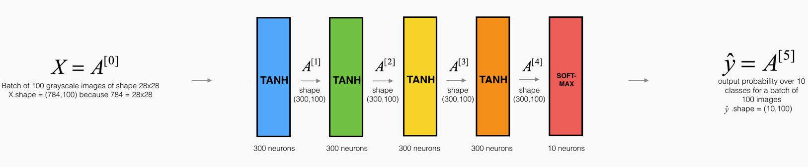
You can find the theory behind this visualization in Glorot et al. (2010). The next section presents the mathematical justification for Xavier initialization and explains more precisely why it is an effective initialization.
IV Justification for Xavier initialization
In this section, we will show that Xavier Initialization keeps the variance the same across every layer. We will assume that our layer’s activations are normally distributed around zero. Sometimes it helps to understand the mathematical justification to grasp the concept, but you can understand the fundamental idea without the math.
Let’s work on the layer $l$ described in part (III) and assume the activation function is $tanh$. The forward propagation is:
The goal is to derive a relationship between $Var(a^{[l-1]})$ and $Var(a^{[l]})$. We will then understand how we should initialize our weights such that: $Var(a^{[l-1]}) = Var(a^{[l]})$.
Assume we initialized our network with appropriate values and the input is normalized. Early on in the training, we are in the linear regime of $tanh$. Values are small enough and thus $tanh(z^{[l]})\approx z^{[l]}$, meaning that:
Moreover, $z^{[l]} = W^{[l]}a^{[l-1]} + b^{[l]} = vector(z_1^{[l]},z_2^{[l]},\dots,z_{n^{[l]}}^{[l]})$ where $z_k^{[l]} = \sum_{j=1}^{n^{[l-1]}}w_{kj}^{[l]}a_j^{[l-1]} + b_k^{[l]}$. For simplicity, let’s assume that $b^{[l]} = 0$ (it will end up being true given the choice of initialization we will choose). Thus, looking element-wise at the previous equation $Var(a^{[l-1]}) = Var(a^{[l]})$ now gives:
A common math trick is to extract the summation outside the variance. To do this, we must make the following three assumptions:
- Weights are independent and identically distributed
- Inputs are independent and identically distributed
- Weights and inputs are mutually independent
Thus, now we have:
Another common math trick is to convert the variance of a product into a product of variances. Here is the formula for it:
Using this formula with $X = w_{kj}^{[l]}$ and $Y = a_j^{[l-1]}$, we get:
We’re almost done! The first assumption leads to $E[w_{kj}^{[l]}]^2 = 0$ and the second assumption leads to $E[a_j^{[l-1]}]^2 = 0$ because weights are initialized with zero mean, and inputs are normalized. Thus:
The equality above results from our first assumption stating that:
Similarly the second assumption leads to:
With the same idea:
Wrapping up everything, we have:
Voilà! If we want the variance to stay the same across layers ($Var(a^{[l]}) = Var(a^{[l-1]})$), we need $Var(W^{[l]}) = \frac{1}{n^{[l-1]}}$. This justifies the choice of variance for Xavier initialization.
Notice that in the previous steps we did not choose a specific layer $l$. Thus, we have shown that this expression holds for every layer of our network. Let $L$ be the output layer of our network. Using this expression at every layer, we can link the output layer’s variance to the input layer’s variance:
Depending on how we initialize our weights, the relationship between the variance of our output and input will vary dramatically. Notice the following three cases.
Thus, in order to avoid the vanishing or exploding of the forward propagated signal, we must set $n^{[l-1]}Var(W^{[l]}) = 1$ by initializing $Var(W^{[l]}) = \frac{1}{n^{[l-1]}}$.
Throughout the justification, we worked on activations computed during the forward propagation. The same result can be derived for the backpropagated gradients. Doing so, you will see that in order to avoid the vanishing or exploding gradient problem, we must set $n^{[l]}Var(W^{[l]}) = 1$ by initializing $Var(W^{[l]}) = \frac{1}{n^{[l]}}$.
Conclusion
In practice, Machine Learning Engineers using Xavier initialization would either initialize the weights as $\mathcal{N}(0,\frac{1}{n^{[l-1]}})$ or as $\mathcal{N}(0,\frac{2}{n^{[l-1]} + n^{[l]}})$. The variance term of the latter distribution is the harmonic mean of $\frac{1}{n^{[l-1]}}$ and $\frac{1}{n^{[l]}}$.
This is a theoretical justification for Xavier initialization. Xavier initialization works with tanh activations. Myriad other initialization methods exist. If you are using ReLU, for example, a common initialization is He initialization (He et al., Delving Deep into Rectifiers), in which the weights are initialized by multiplying by 2 the variance of the Xavier initialization. While the justification for this initialization is slightly more complicated, it follows the same thought process as the one for tanh.
Learn more about how to effectively initialize parameters in
Course 2 of the Deep Learning Specialization
Examples include Adam, Momentum, RMSProp, Stochastic and Batch Gradient Descent methods.
A neural network with two hidden relu units and a sigmoid output unit.
Mean is a measure of the center or expectation of a random variable.
Variance is a measure of how much a random variable is spread around its mean. In deep learning, the random variable could be the data, the prediction, the weights, the activations, etc.
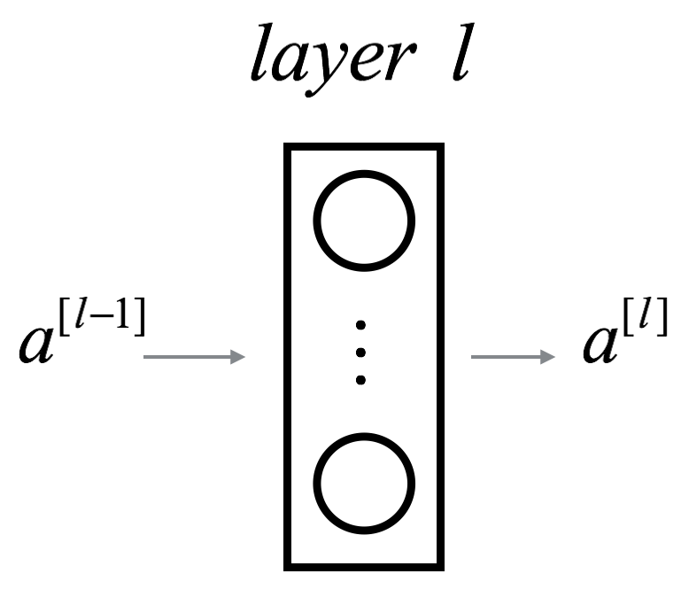 $a^{[l-1]}$ represents the input to layer $l$ and $a^{[l]}$ represents the output. $g^{[l]}$ is the activation function of layer $l$. $n^{[l]}$ is the number of neuron in layer $l$.
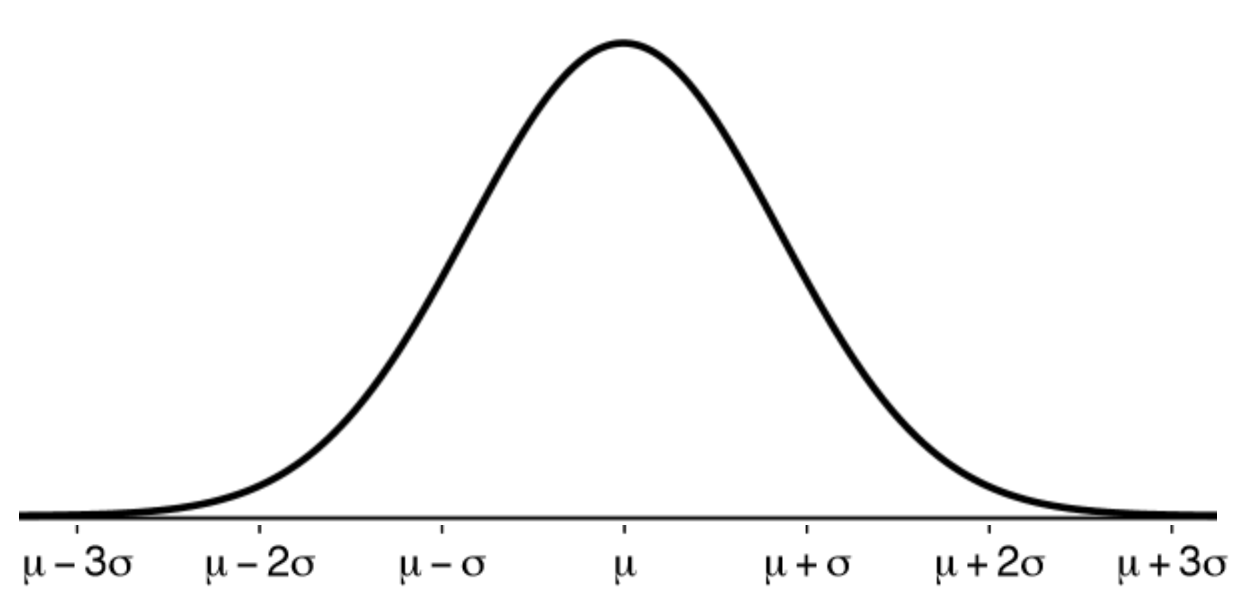 Values generated from a normal distribution $\mathcal{N}(\mu,\sigma^2)$ are symmetric around the mean $\mu$.
$a^{[l-1]}$ represents the input to layer $l$ and $a^{[l]}$ represents the output.
$tanh$ is a non-linear function defined as $tanh(x) = \frac{1 - e^{-2x}}{1 + e^{-2x}}$.
Important properties of $tanh$ are its parity ($tanh(-x) = -tanh(x)$) and its linearity around 0 ($tanh'(0) = 1$).
The variance of the vector is the same as the variance of any of its entries, because all its entries are drawn independently and identically from the same distribution (i.i.d.).
These assumptions are not always true, but they are necessary to approach the problem theoretically at this point.
This is only true for independent random variables.